With a few steps you will learn how to perform them within your project in Excel, to be able to make any percentages chart, advanced equations and increments within your text to bring it professionally. You should also know that in Excel you can also create speedometer charts and insert charts using the repeat function.
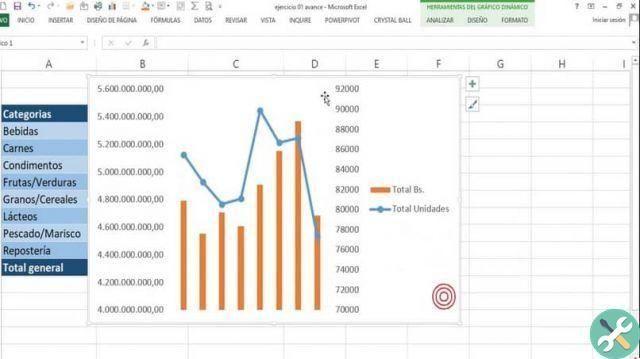
How to create an advanced curved line chart in Excel?
- First we need to go into Excel and from there be able to create this advanced chart on a percentage or on different digits.
- If we have the figures already positioned inside the different Excel cells, we will enter the «Insert» tab and then we will look for the option "Line graph".
- There an option will appear in which we see several options to create the line chart, in this case we will use linear ones in 2D.
- When we click on the 2D line graph option, the graph will automatically appear in our project, to change the lines and give them a curved movement we need to configure the lines.
- To configure the lines we have to click with the right mouse button on a line of the graph, a menu is displayed that offers us the option "Data series format ...".
- Within Excel a side menu appears in which it provides us with the editing options, we have to click on the "Fill and Line" option which appears as a "paint bucket" icon and when we click, different options will be displayed to modify.
- We need to select the option "Smooth line" which will provide us with the curves in the lines within the newly created chart and thus will be able to give the curved appearance within the chart.
- Within this menu we can change not only the line and its format, but also its size and width as the default color for our chart in Excel.
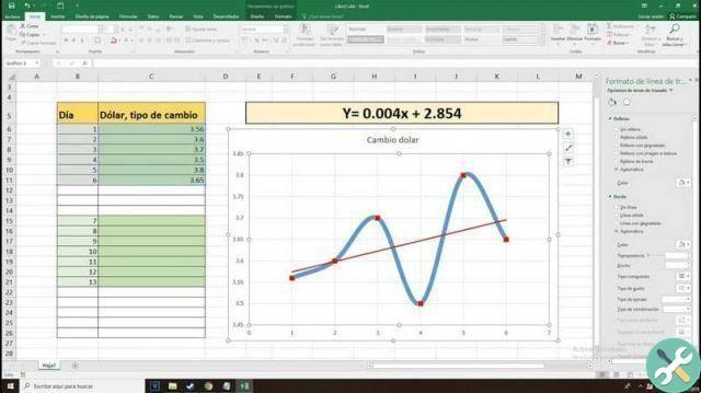
How to create a line equation and add trend line in Excel?
- To do this we need to create a new document in Excel, then create two columns and in one place "X" and in the next column place "Y" to be able to graphically position the figure of the equation in each point under each column.
- With these figures we will create the graph in the equation, we must go to the option «Insert» and search inside it "Graphic" and there a new window will open.
- There in the new window where we will choose which type of chart we will use, in this case we will select the option "XY (dispersion)" and we can see that not only do we have this chart option, but it also allows us to exhibit ourselves as column, bar and circles, among others.
- We will mark the points and lines that we will need for the graph and then we will check «Finish».
- This way we will immediately have the chart in our spreadsheet.
- To be able to edit this graph we must double click on the same graph and inside the row we will click with the right mouse button, where the menu is displayed.
- And they will place the "Insert Trendline" option.
- A new window will open where it will allow us to make changes to this new line, we will go to the "Type" tab and there we will choose the linear function, select the option "Show equation".
- By clicking on «OK» we will see that our chart will change and a new line will be added, in this way you can modify and add the trend lines that you are interested in displaying in your project chart.
With these techniques explained step by step you can give a professional and more comfortable format to your work projects, create advanced graphics in Excel DON'T è never been easier. Don't miss the most comprehensive Excel guides inside miracomosehace.com
TagsEccellere