How to create an interactive donut chart in an Excel sheet
To follow the following tutorial, you need to have a table with the various data already established or create a pivot table in Excel. Likewise, we recommend that you use the donut chart only in tables that don't contain too much data.
To insert an interactive donut chart into an Excel sheet, follow these steps:
- Once the whole board is complete, you can apply a donut chart, which will greatly improve the look of your board.
- The process for inserting a donut chart is quite simple in the latest versions of Microsoft Excel. The first thing to do is to go to the section of insertion, located in the options section at the top of the screen.
How to create an interactive donut chart in an Excel sheet" src="/images/posts/a7a8227b53648e9fdced90179279a761-0.jpg">
- Find the section graphics, specifically you have to click on the option of the graphics with a circular shape.
- In this section various options will be shown, the one you are interested in this time is ring, click on it rings.
- The chart should appear in your Excel table, positioned in the place that seems most comfortable to you, in the same way you can change its size.
- Once you're happy with the table's appearance, right-click on it. All options related to this graph will appear on the screen, you need to click select data ...
- A dialog box about the data in the table will appear. At the top is the data range of the chart. Click this option and select all the data you want to include in this donut chart, click the accept option.
After the above steps, you will have the foundation of your ring-shaped artwork. In any case, if you don't like the final overall look, you can configure it to your liking by inserting a legend to the Excel chart or by following some of the steps we will mention below.
![<a name=]() How to create an interactive donut chart in an Excel sheet" src="/images/posts/a7a8227b53648e9fdced90179279a761-1.jpg">
How to create an interactive donut chart in an Excel sheet" src="/images/posts/a7a8227b53648e9fdced90179279a761-1.jpg">
Customize the graphics of the ring
The ring-shaped graphics are quite attractive and very intuitive, using it will highlight the look of your board a lot, but you can go further. In fact, you can improve the appearance of Excel charts and the donut chart is no exception to this rule. To change the formatting options within this chart, follow these steps:
- If you want to customize the donut chart you created earlier, right click on the ring.
- The options related to the graph will appear on the screen, click on the option to format the data series.
- A new panel will appear on the right of your screen that you can configure to your liking, use the different options that will appear there according to your tastes, in this way you can give a personal touch to your new graphics.
- As a final section, remember that you can have your chart have an automatic update in Excel, something highly recommended for most charts of any nature.