Step by step you will learn how to compare lists in excel, it will help us to know if the content we find in another list is repeated in one of these, compare large Excel lists to see what repeats will no longer be a headache, you can do it in minutes with this option.
How to compare lists in Excel?
- To start you must install Excel on your PC.
- First we need to create a new text document inside Excel that it is empty.
- Within it we will create two lists of what you need to do in your project.
- To compare these two we must first have prepared the lists with their already defined numbers / digits.
- Let's select all the cells from the first list.
- In the top menu we will find the “Start” tab and then in the “Conditional Formatting” option which displays a new menu of options.
- We select the option in the menu "New rule" to open a new window where we can choose the configurations for this new rule.
- The configuration we will choose will be "Use a formula that determines cells to apply formatting" within this we have to create a formula in the section within the same window.
- We will write the following: = COUNTIF, in brackets we will select the next line of our list with which we will compare, then we will add a ";" and when we are done we select the first cell of our initial list again.
- In this selection, put a $ sign twice, we will remove them from our formula.
- We close the brackets and continue the formula with ">" and the value "0".
- We can select the option "Format" before accepting the formula, we can model it within it.
- We will change our text style to “Bold” and we will give colorful background if needed.
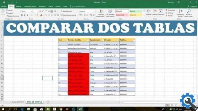
When we accept, we will see the numbers repeating in the second list reflected in the first list. In this way, it will be with the background of the color we have chosen and with the letter highlighted in "Bold".
Important: This formula is created when the action is performed, we cannot save the formula within Excel to be able to use it later in another project, spreadsheet in that program.
Keep in mind when comparing two lists in Excel:
This configuration can be used to search for digits / numbers within a long list of numbers, where it is impossible to manually review them one by one and would take many hours.
We can use this example not just with a list of numbers, we can also add a single number / digit to our formula to look up in the list and that way we focus on a single number. A very useful tool you learned in this step by step, how to compare two lists in Excel and repeat highlighting. You may also be interested in learning more about how insert formulas into text boxes in Excel, in case it is necessary to do so.
We can perform the same procedure but vice versa to obtain the same search but in the next list, it is important to note that the previous search will not be altered by this new formula to be defined between the second list compared to the first list.

Excel shows us once again that it is a powerful editor / creator of documents in spreadsheet format, with its tools it manages to generate the user a 100% probability that his project, table or spreadsheet will be successful. Although we also have alternatives to create a spreadsheet in a professional way.
Remember that to access Excel more step by step, you need to enter the main menu of the page and search for the Excel label where you will find everything about this wonderful program, how to get total and subtotal in Excel, how to do logic functions in Excel and much more.