Many times you've asked yourself this question, come on how to change the color of a cell and what function does Excel have to solve it. But unfortunately the functions don't change the appearance of the cells, they change the data those cells contain. That is why in this case we will use a format to solve it.
Yes, as you can see, we will use the conditional format present in the Excel options. And this will help us in a simple way to solve this problem, if you realize that a format will allow us to change the appearance of our spreadsheet. Unlike what it would do if we used a function.
If we have a table composed, for example, of 6 columns and 20 rows, we could use a function to freeze the rows and columns. But you couldn't find a function that allows us to set or change a row color based on text or cell value in Excel. We will then explain how to apply this format in the data table.
How to change the color of a row based on the text or value of a cell
To perform this explanation, you need to have your Excel sheet ready with a table that contains multiple columns, for example five. And with more lines like 10, this data can contain any information, the important thing is that you learn how to change the appearance of cells using conditional formatting.
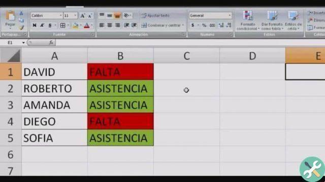
Continuing with the example, suppose our table shows us six columns with the following data: Product, quantity, value, total, condition. Where will the condition be whether the product has been canceled or not. And the lines represent the 10 products marketed in the sector.
So we want color the lines with some color containing products that have not been deleted. To do this non-manually, we need to use the conditional format. We do this in the following way, select the whole table and then go to the Home tab, to change the color of a row in Excel.
Conditional format
In this tab we will look for the option Conditional formatting, bring up a clip and other options and choose New rule. When you crop, a window will appear with the name New Formatting Rule. In it there are several options but we will choose «Use a formula that determines the cells to apply the formatting.
When choosing this option, we must then write the formula we will use, the formula would be as follows = $ E4 = "Not canceled". This formula means that all cells that are in column E, which is the condition column, that is, whether a product has been canceled or not. From the first cell or E4 to the last and only those with this Not Canceled message will have a color.
Then you need to press the format button, here you can select the color you want the cells with the message Not cleared to have. You can also change the look, add an effect, change borders, choose patterns, and more. Then you have to accept everything and your box will present the color you have chosen, in the cells that have the message of Not canceled.
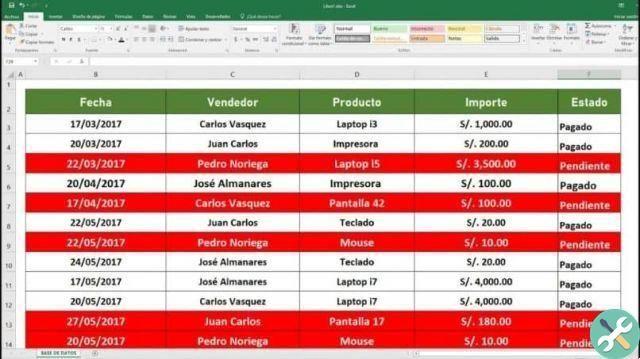
And this same format can be applied to the rest of the table, but now applying the formula to the cells that have the Canceled message. Where, for this message, only the color will change. And in a very simple way you learned how to insert or change a row color based on text or cell value in Excel.
TagsEccellere