How do you calculate the annual growth rate in Excel?
The calculation of growth percentages takes place automatically and very practical only with the application of formulas. There are many ways to do the calculation, but this is the simplest formula to apply.
- % Growth = ((present value - previous month value) / (previous value)
When you apply this formula in Excel to the cell where you want to display the percentage results, the operation will be done.
- = ((B3-B2) / B2)
B2 represents the value obtained from the previous month, which is the cell preceding the month under evaluation. Cell B3 represents the current balance, whose growth percentage you want to evaluate.
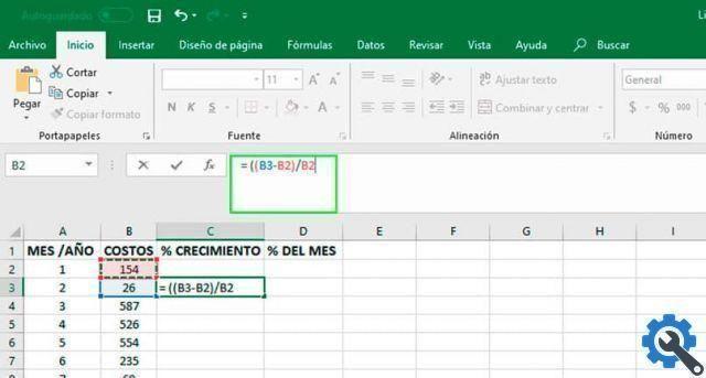
Note: To see the percentage value in the cell, you need to change the format to percentage. Right click on the cell, select the Format Cell option and finally select the percentage category.
Alternative formula (NO.PER or XIRR function)
Usually this formula is used for regularly assess the value of cash flow. The meaning of its syntax is TIR.NO.PER and it means “values.date.estimate”. In case the Excel version is in English, the function name is XIRR.
- Values: is the range of data used to measure the rate.
- Date: data evaluation period.
- Pixy: is optional and is used to find an estimated value close to the IRR.
All aggregated values must have a minus sign (-) at the end for the calculation to be successful. Applying this formula in Excel would look like this:
- = TIR.NO.PER (B2: B13; C2: C13)
Where column B represents the value and column C represents the date.
Finally, you can calculate the average of the results obtained by comparing the result of a month with other values monthly. It is a predefined function available and can only be accessed by writing the word average and entering the values to be calculated.
- =MEDIA(B2:B13)
Calculation of the average of each month compared to the total
Once calculated the total sum of all the values to be evaluated, it is possible calculate the percentage of sales made in that period of time over the entire year. The formula is as simple as the one used to calculate the mean. The total sum of annual sales is divided by the grand total of sales for that month.
- = B2 / $ B $ 14

Final report: the sum calculation formula is simple = Sum (B2: B13). What is stated in this formula is that the sum of all values between B2 and B3 must be done.
Add graphic icons
To show the results in a more graphic and understandable way to the naked eye, you can add colored arrow icons. Each arrow has a meaning, if it is green and upwards it means that there has been a growth in sales, if it is yellow there have been no changes compared to the previous period and if it is red and downwards it means that there have been losses.
To apply this change it is necessary add another formula in another cell. The result obtained by the formula alone is 1 = there was growth, 0 = remains the same and -1 = there were losses. You have to start from the second period, because the first month is unmatched.
- = SEGNO (B3-B2)
Then select the result obtained in all cells and from the Home tab click on the option Conditional formatting. Select the icon set you prefer and the changes will be applied immediately.
To remove the numbers next to the icon is required change the formatting rules, from the same option Conditional Formatting you can manage the rules. Select only show symbol, apply the changes and everything will be perfect.