A disorganized worker could lead to an entire office malfunction, causing you to get fired or get your attention. Therefore, we will teach you how to create or create a gantt chart in excel, step by step, quickly and easily.
Plus, if you master tools like Microsoft Excel, you'll have more value for your business. How come? Well, what happens is that companies consider the training in the area of office automation when they evaluate their employees.
As long as you are able to manage these resources, you will promote greater efficiency and work rate. So, don't just follow this guide, take a moment to study other tutorials. In fact, you can even use the Gantt chart to organize the time spent studying.
To follow this article step by step, you need to download and install the Excel software from its official website. Remember that it is a paid program, which you can get from Microsoft's website, however you can purchase a free version.
It makes sense that you have doubts about buying or not, but let me tell you it is a great investment. If you train, there will be an opportunity to hire better locations in your office. Gradually you will get that money back.
What is a Gantt chart?
Gantt charts are graphics tools in able to show us, quickly, the time we have to dedicate to one or more activities, in a certain period already established.
Not only are they an easy way to get organized, they are also extremely easy to do. By mastering the basics of a worksheet or spreadsheet, anyone can design their own Gantt charts.
How to make or create a Gantt chart in Excel?
First, you need to open the Excel spreadsheet to practice while reading the steps. Now, you will create a table in Excel with four columns, and whose names must be: activities, Start end, duration. You can choose the number of cells in the columns, depending on how many activities you want to represent in the diagram.
Select the columns and go to the start context menu. Use the option Bordi, so that our table can be easily established and viewed.
Fill in the cells with the information in the respective columns. Enter the different activities you will do, their start and end dates. You can then manually enter the duration in days for each activity or use a formula = (End-Initial) +1 and apply it to all duration cells.
Now that you have completed the table, you will choose the cell next to the Duration and enter the number 1. In the next one, the number 2. Then leave both (1 and 2) selected and drag the small square that appears in the corner from cell 2, to right. Move it as many cells as there are days of work you want to represent in the diagram.
Select the column where you placed the 1 by tapping the corresponding letter of the coordinates. Use the right mouse button and choose the option Column width to change it, enter a width of 5 and accept.
Drag and applies the same formatting to all other numbered columns. When you're done, select this whole new table with numbers in the columns and apply the outer borders.
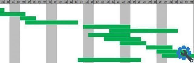
Finally, color the one using the shading option. You will do it in based on the duration value for each activity, so that it looks something like the following image.

That would be all. Now it's your turn. Put the "creative mode" and draw the diagram in the best possible way.