But why this difference between function and format? The difference is that Excel functions are only used to change the different data contained in a specific cell. While a format will change the appearance of said cell. For this reason, if we want to change the color of a cell, we will use a format instead of a cell.
In the world of Office Automation it is important to know these differences and, above all, to know how the different functions and formats of Microsoft Exel work and how they are used. In the following tutorial we will show you the steps you need to follow so that you know how to insert or change color in a cell based on text in Excel, Excel conditional formatting.
How to insert or change color in a cell based on text in Excel - Excel Conditional Formatting" src="/images/posts/d227747fb378fcb11f331e80ebafa953-0.jpg">
How to insert or change color in a cell based on text in Excel
As we have already explained, we will not use an Excel function other than a format, in our case the Conditional Format. For this we will go to the Excel program and then open a new spreadsheet that you can name. If we already have a table with the saved data we can open it, if not, we start from scratch to create our data table.
For this example we can insert in a small table with 7 columns and 5 rows, in the columns we will place the invoice number, the date, the amount, the product description, the quantities, the total price and the payment condition. In case of cancellation or not, the data of 5 invoices that have been made will be entered in the lines.
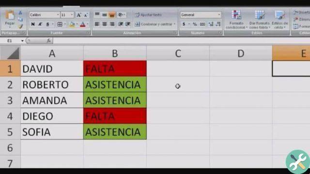
We finish entering the data in our table and we will place that in lines 1, 3 and 4 the invoice is canceled or paid. In the other two lines which are lines 2 and 5, the invoice has not yet been canceled. Now we want the lines where it appears not deleted are colored red and the lines where it appears deleted are colored green.
To do this, we will select the entire table so that all its data is highlighted, then we will go to the top menu. And we will select the Home tab and then we will create a clip in the option Conditional formatting. In this way, several options will appear and we will choose New rule. It should be noted that you can also select a range of cells in Excel with keyboard shortcuts.
Enable conditional formatting
A small window will appear and in it we will choose the option «Use a formula that determines cells to apply formatting. Let's make a clip and then we'll write the rule, this is it = $ G3 = "canceled". With this rule we are saying that the lines containing the deleted value turn green.
For this we create a clip in the Format option, here a new window appears and we will choose the color, in our case green, then we will click OK. Then it will take you to the previous window and again you need to click OK. And you will appreciate that in all those lines that have the value cleared have been changed to green.
In our example they will be lines 1,3 and 4, so we will have to repeat the same procedure for the lines that have the value "not deleted" and instead of green you will put the color red. And so you will see how your table will change the color of the rows where, based on the information it has, it will give us a different color.
How to insert or change color in a cell based on text in Excel - Excel Conditional Formatting" src="/images/posts/d227747fb378fcb11f331e80ebafa953-1.jpg">
And in this way you learned how to use a very useful format for making changes to the appearance of cells. And with this tutorial you can learn how to insert or change color in a cell based on text in Excel, Excel conditional formatting.
TagsEccellere