Why freeze rows and columns in Excel?
The main reason is that when you create spreadsheets in Excel, the information is emptied into tables whose row or column headings (usually the first ones) you need to know or have as a constant reference, in other words it is must always have them in sight.
This occurs when, for example, the information in the spreadsheet is very extensive and not all of the information is displayed on the screen. In these cases, there is no other choice than scroll through the document using the mouse or the side scroll bars, moving up or down to view the information on the screen.
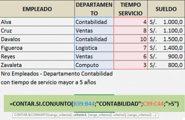
If you are clearing information from a list or want to insert multiple rows or columns in Excel with macros, constantly moving the sheet to see the references of the first columns or rows can get very tiring. Therefore, it is very useful keep the required area visible on the screen even if you insert new columns or move through the document.
Steps to freeze rows and columns in Excel
Before we start, it is useful to note that Excel also allows some very large sheets, it is better to filter the tables with Range.Autofilter to solve the problems we talked about.
Below we show you the steps to follow to be able to freeze rows and columns in Excel, taking into account that the procedure to follow is very similar for each case.
Case 1: freeze the first row
To be able to freeze the first row of a table, simply follow these steps:
- vai to the view option on the toolbar and select it.
- Press the option for lock the panels.
- Press the option for freeze the first line.

Case 2: freeze the first column
To be able to lock the first column of a table, simply follow these steps:
- vai to the view option on the toolbar and select it.
- Press the option for lock the panels.
- Press the option for lock the first column.

Case 3: Freeze the panels
It's possible split sections or panels of the worksheet resulting in two or more independent areas within which the user can scroll, while the rows or columns of the non-scrolling area remain visible.
The above is one variation of cell blocking or freezing in Excel and to freeze more than one column or row of a table (panels), just follow the following steps:
- Go to the toolbar option or tabbed view and select it.
- Press the option or lock the panels.
- The cursor must be located under the lines you want to freeze e to the right of the columns you want to freeze, this will freeze all rows above the selected cell, and all columns to the left of the selected cell.
Steps to mobilize cells in Excel
reverse the previous steps, i.e. in order to have our full spreadsheet window again without fixed cells, just select the ones that are locked, follow the following steps:
- Go to the toolbar option or tabbed view and select it.
- Press the option or tab to mobilize the panels.
That's it, if you follow these steps you will be ready to save and print your Excel tables and spreadsheets. Very easy, right?
As you have seen, it is not very difficult to freeze the cells in an Excel spreadsheet, you have already learned everything that is needed to get it. On the other hand, keep in mind that correcting columns or rows in Excel only affects how it looks on the screen. They will not change their original position within the spreadsheet.
So, take the opportunity and start making your projects in Excel using the new tricks and shortcuts learned so you can finish them faster and more efficiently.


